Variational Autoencoders are Beautiful

Steven Flores
Monday, Apr 15, 2019

The variational autoencoder is one of my favorite machine learning algorithms. It does it all: finds low-dimensional representations of complex high-dimensional datasets, generates authentic new data with those findings, and fuses neural networks with Bayesian inference in novel ways to accomplish these tasks.

The autoencoder

To understand a variational autoencoder, we can study its probabilistic underpinnings [1, 2]. However, it may be easier to understand at first as an adaptation of an “autoencoder.” [4–6]. We take this approach here.

Data compression

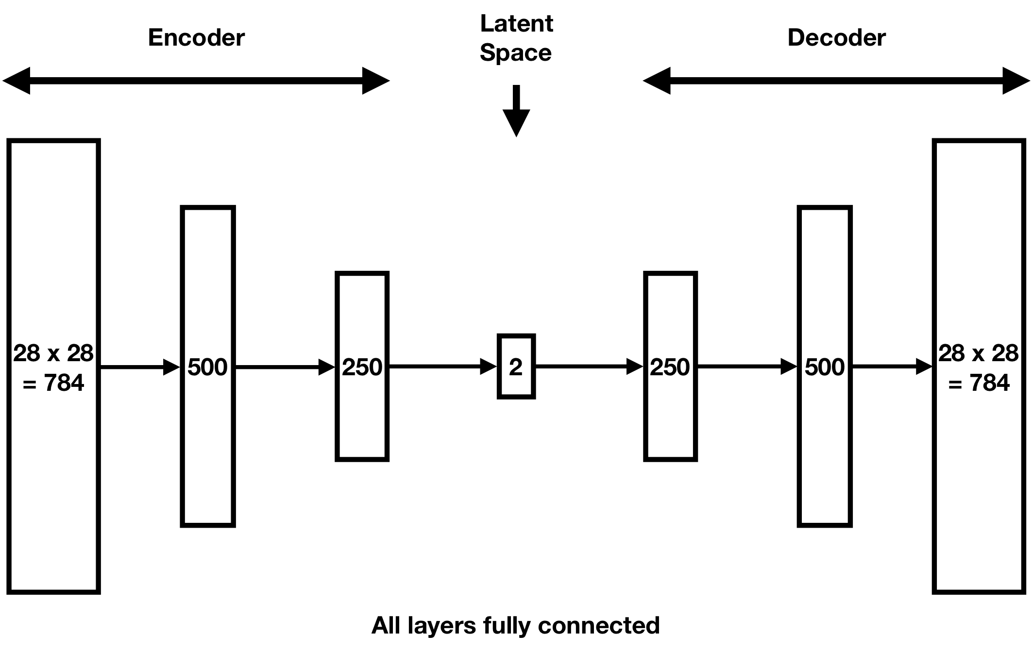
An autoencoder is a lossy data compression algorithm. Its macro-architecture comprises an “encoder” followed by a “decoder.” The encoder E maps a point x in our dataset to a new point E(x) in a low-dimensional “latent” space. The decoder D maps E(x) to a second new point D(E(x)) in the original high-dimensional space containing x. Usually, E and D are neural networks, often with ReLU activation functions. Here is a diagram of this architecture:

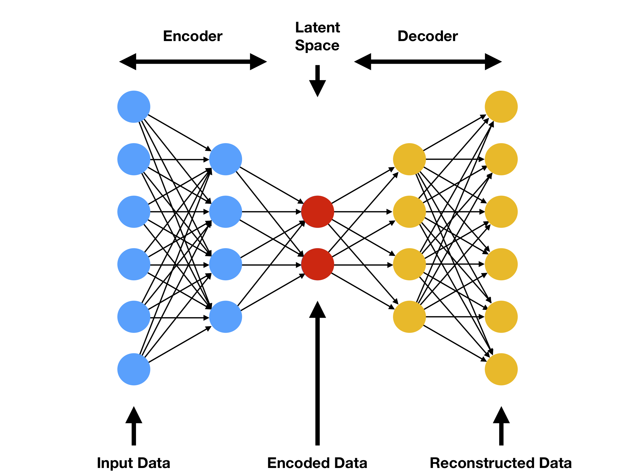
The autoencoder loss function sums the differences between each point x in some training dataset and its reconstruction D(E(x)). If the loss is small when summed over a validation dataset instead, then the decoder D does well at reconstructing an arbitrary datapoint x from its compressed image E(x).

Data generation

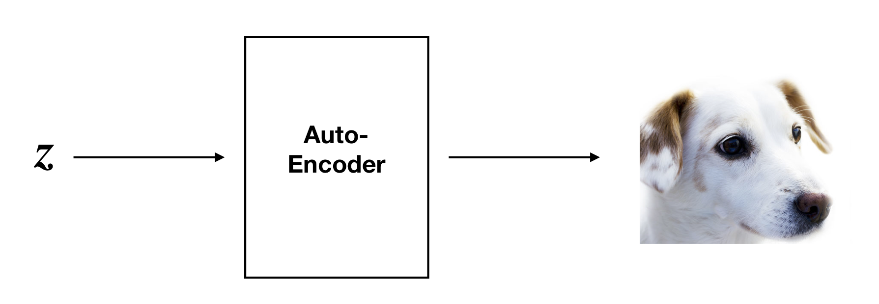
Now we consider a tempting application: data generation. Feeding a vector z from the latent space into the decoder generates a new “fake” datapoint D(z). We want D(z) to be similar to other points in our original dataset. For example, if we are working with image data, then it would be nice if we could discover a vector z such that

But it may be more likely that z generates nothing like points in our dataset after passing through the decoder D:

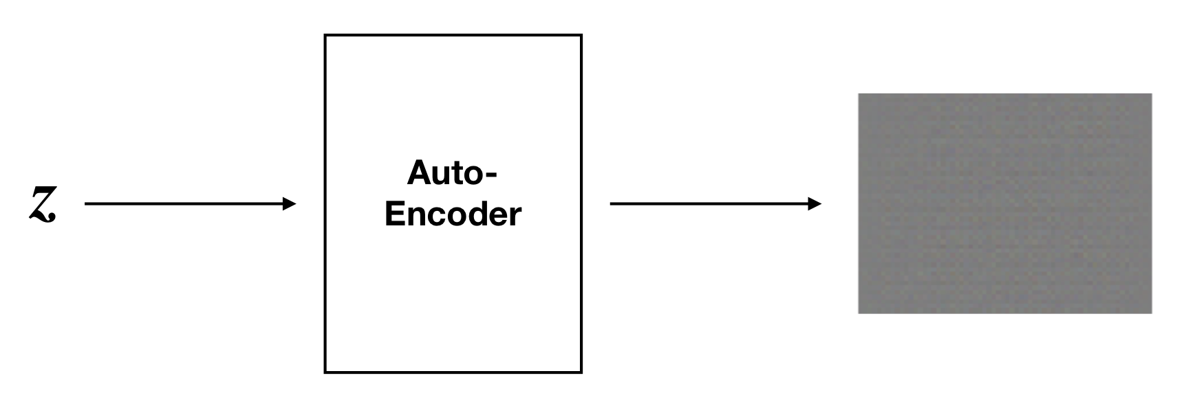
This begs the question, how do we sample values for z that produce high-quality imitation data?

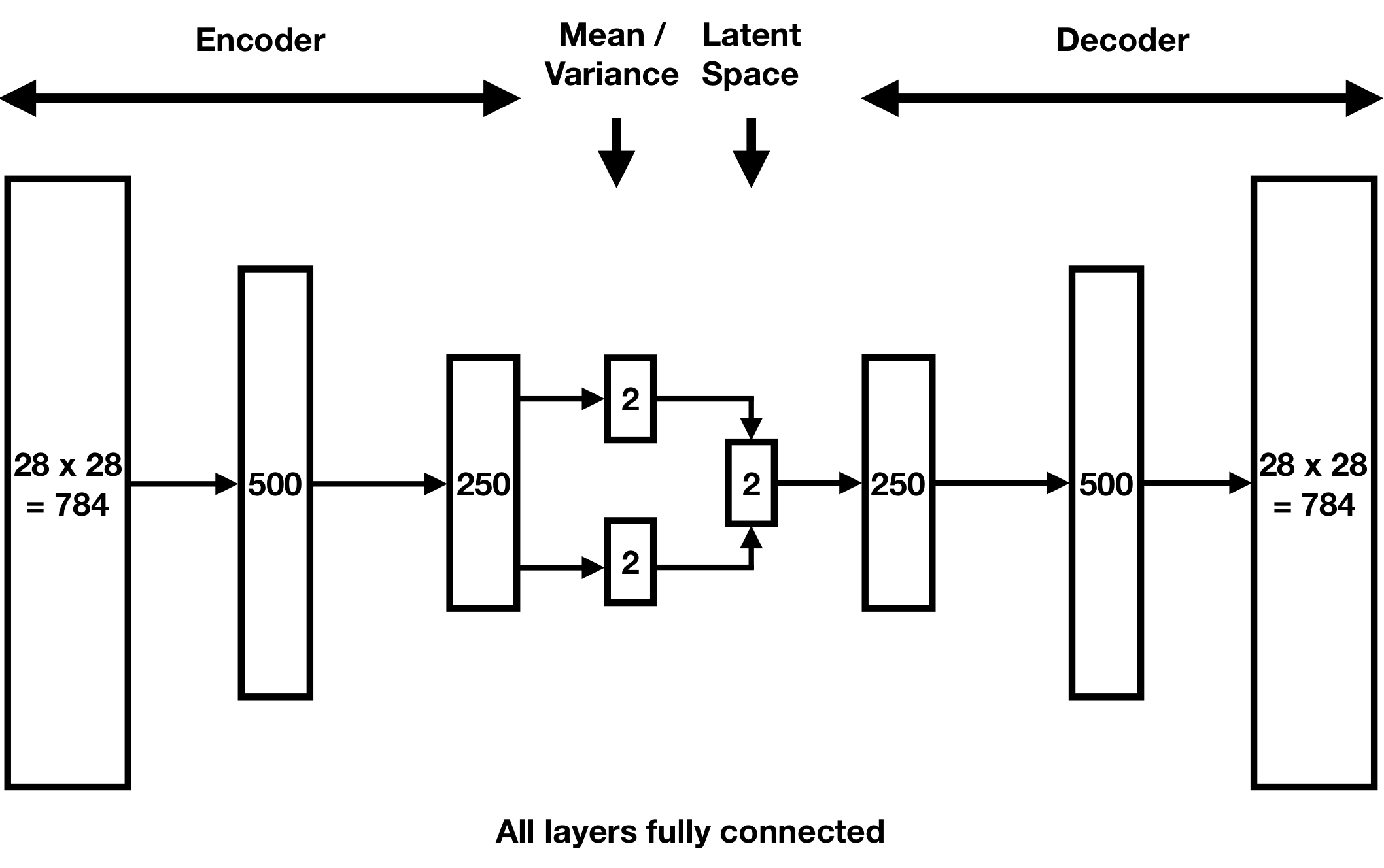
We showcase these difficulties using an autoencoder that compresses the famous MNIST 28 × 28 handwritten digits dataset [7]. We use the following neural network architecture, which has a two-dimensional latent space:

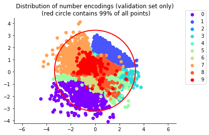
After training our autoencoder (by minimizing its loss function via stochastic gradient descent), we find these encodings of the handwritten digits in our validation set, grouped by their labels 0–9:

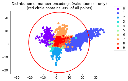
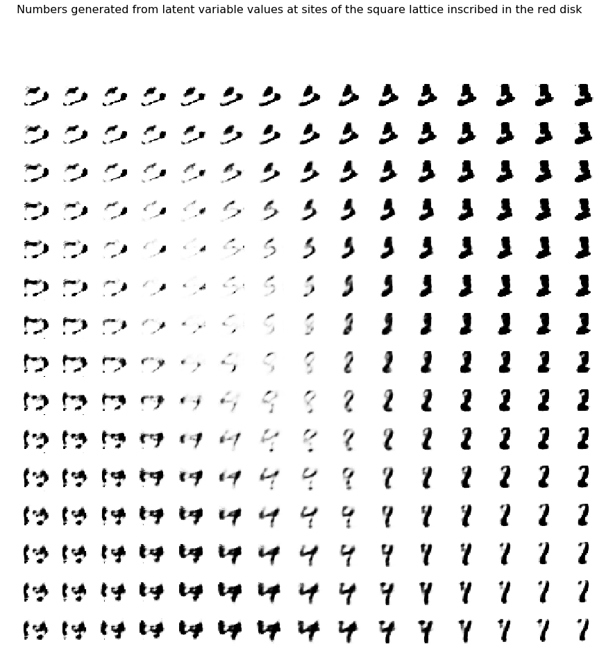
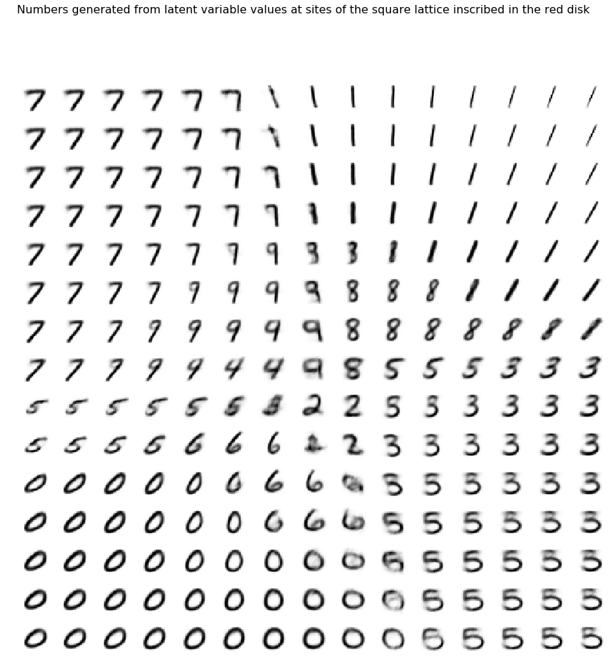
The red circle is concentric with and encloses 99% of the encodings in the point cloud. The shapes of these clusters are complicated, making them hard to sample. Indeed, if we inscribe in the red circle a square lattice,

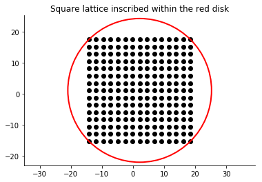
and pass the vector at each lattice site through the decoder, then we generate the following “fake” handwritten digits:

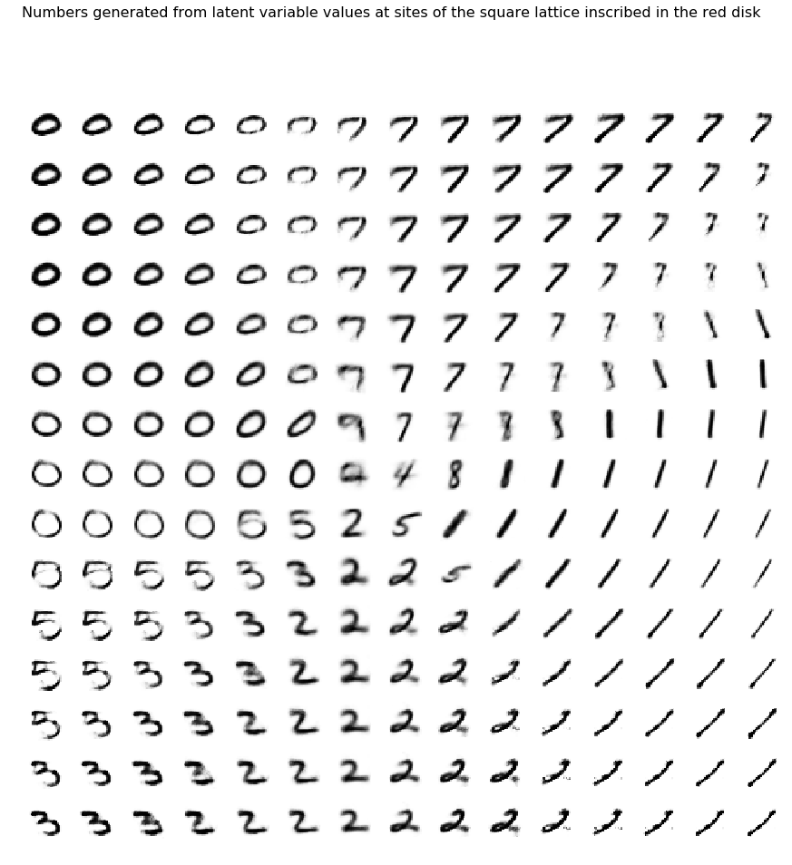
While many images have good quality, others are blurry or incomplete because their sites are far from the point cloud.

A ten-dimensional latent space enhances this problem. Here, a ten-dimensional hypersphere now surrounds a ten-dimensional point cloud. We generate these “fake” digits from lattice sites in the great circle slicing the hypersphere in the plane of the first two coordinates:

The quality of the generated handwritten digits is worse than in the two-dimensional case. Because two-dimensions is usually too small to capture the nuances of complicated data, this is not good news.

The variational autoencoder

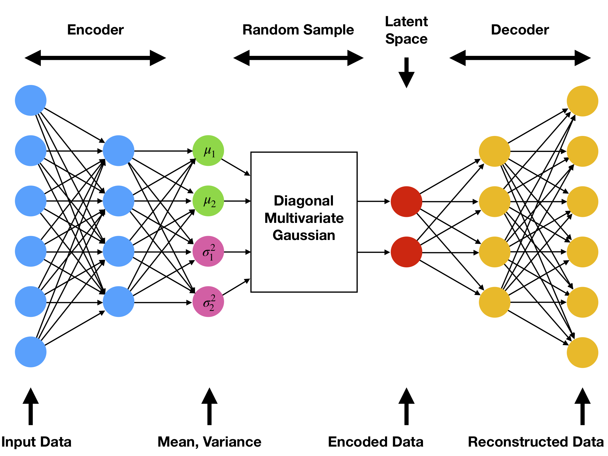
We can fix these issues by making two changes to the autoencoder. The result is the “variational autoencoder.” First, we map each point x in our dataset to a low-dimensional vector of means μ(x) and variances σ(x)² for a diagonal multivariate Gaussian distribution. Then we sample that distribution to obtain the encoding E(x):

Second, we add an extra term “KL-divergence” [8] term to the loss function that clusters encodings into a hypersphere.

Data generation

Now we repeat our MNIST example for handwritten digit generation with a variational autoencoder. Using a two-dimensional latent space, our architecture is as follows:

After training, here are the two-dimensional means μ(x) of the handwritten digits x in our validation set:

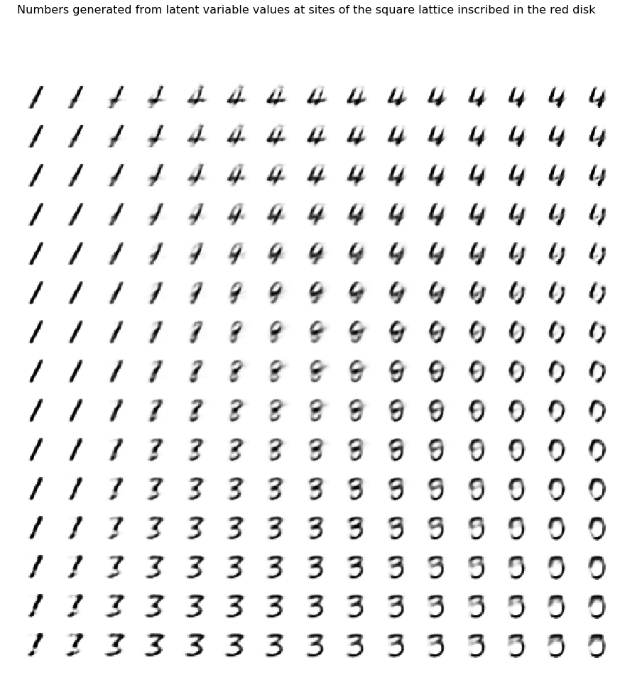
As desired, the means are clustered in the shape of a disk. Sampling the same lattice sites as before, we now generate these realistic “fake” handwritten digits:

Indeed, these results outperform the plain autoencoder, but the images are blurry. We see more improvement with the ten-dimensional latent space. Working with the plain autoencoder, we generate these “fake” handwritten digits:

These results outperform the plain autoencoder even more, but the images are still blurry. In general, variational autoencoders outperform plain autoencoders at the task of data generation.

Data interpolation

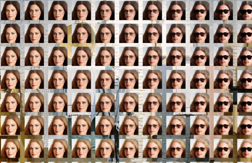
Variational autoencoders give us another useful capability: smooth interpolation through data. To illustrate, we train a variational autoencoder on the CelebA dataset [9], a large dataset of celebrity face images, with label attributes such as facial expression or hair color. We crop and resize these images to size 64 × 64 × 3.

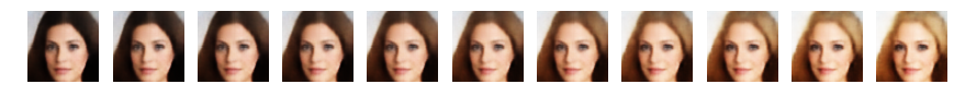
Now we use linear interpolation to, for example, transition hair color to blond as follows. We take the difference ∆ of the center of the set of faces in our training set with blond hair and that of faces without blond hair. Then we add multiples of ∆ with increasing length to a face to gradually change its hair color to blond. For example, we have

Using the same approach, we can also gradually add sunglasses to a face,

or we can gradually add sunglasses and change hair color at the same time:

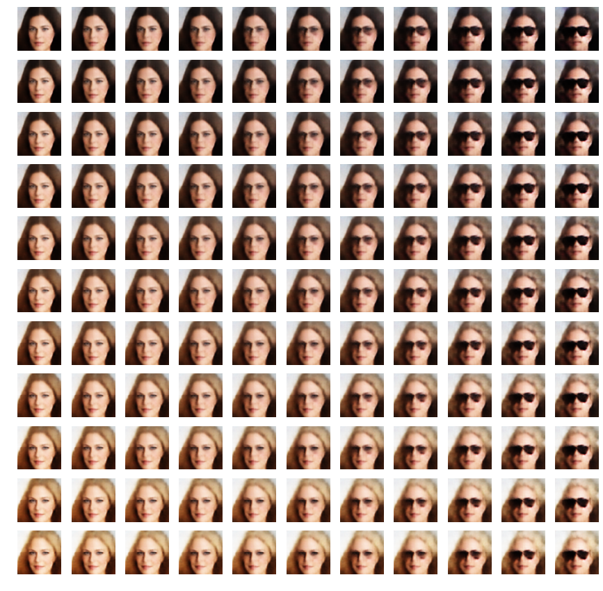
Among all possible 64 × 64 × 3 color images (with 256 possible colors per pixel), the subset of images that display a face is a small fraction. That we can interpolate between two images of faces without leaving this subset is remarkable.

While this capability is impressive, these generated images are quite blurry. Some of this blur can be removed by using a so-called perceptual loss function [10], a discriminator loss function [11], or with other techniques.

Summary and further directions

The ability of a variational autoencoder to generate realistic images by random sampling is impressive. Today, new variants of variational autoencoders exist for other data generation applications. For example, variants have been used to generate and interpolate between styles of objects such as handbags [12] or chairs [13], for data de-noising [14], for speech generation and transformation [15], for music creation and interpolation [16], and much more.

Check out our project on github: https://github.com/compthree/variational-autoencoder. There, you can find our implementation of a variational autoencoder, all of the code that generated the results discussed here, and further details about network design and training that we did not discuss. We welcome all feedback.

Interested in learning more about Variational Autoencoders are Beautiful?
Enter your email below:

Variational Autoencoders are Beautiful

The autoencoder

Data compression

Data generation

The variational autoencoder

Data generation

Data interpolation

Summary and further directions

Share: